
1. Pytorch变量的基础操作
2. Pytorch前向反馈网络的构建
3. 试着跑了一下Pytorch前往网络的反馈
向量化表达
以后打算专门再写一下反向传播,下面两个视频我之前看了觉得对理解这块非常有帮助NerualNetWorkP1NerualNetWorkP2
import torch
import numpy as npdef activation(x):# 记住Torch对于数组的操作形式和Numpy真的差不多return 1 / (1 + torch.exp(-x))np.exp([1,2,3])
# array([ 2.71828183,  7.3890561 , 20.08553692])
torch.exp(torch.arange(0.,4)) # 这里要加个逗号,因为exp方法不支持long变量
# tensor([ 1.0000,  2.7183,  7.3891, 20.0855])torch.manual_seed(7)features = torch.randn((1,5))
weights = torch.rand_like(features)
bias = torch.rand((1,1))
torch.randn()函数构建一个1行5列的Tensortorch.randn_like(Tensor2)构建一个与input tensor形状一样的tensortorch.randn()从一个正太分布中创建单个值.y = activation(torch.sum( features * weights ) + bias # or just (features*weights).sum() + bias)
print(y)tensor([[0.8072]])
torch.mm或者torch.matmul函数不过需要注意的是,矩阵相称需要保证 (n*m) * (m * q) 的性质weights.reshape(a,b)返回一个新的a,b矩阵(有时会改变原Tensor)位置weights.resize_(a,b)就地改变,返回同一个tensor,这个函数如果a,b与原矩阵形状不同的话,会造成信息丢失。weight.view(a,b) 教程上说这个是最好的,返回一个形状为a,b的Tensoractivation(torch.mm(features,weights.view(5,-1)) + bias)tensor([[0.8072]])
可以进一步简化表达成:
让我们用代码来表达一下这个神经网络
torch.manual_seed(7)features = torch.randn((1, 3))
n_input = features.shape[1]
n_hidden = 2
n_output = 1
# 第一层的权重
W1 = torch.randn(n_input,n_hidden)
# 第二层的权重
W2 = torch.randn(n_hidden,n_output)
# 两层的偏置项
B1 = torch.randn(1,n_hidden)
B2 = torch.randn(1,n_output)
接下来计算一下2层的结果输出
h = activation(torch.mm(features,W1) + B1)
output = activation(torch.mm(h,W2) + B2)
print(output)tensor([[0.3171]])
torchvision把这个数据下载下来import numpy as np
import torch
import matplotlib.pyplot as plt
%matplotlib inline
%config InlineBackend.figure_format = 'retina'
from torchvision import datasets, transforms
transform = transforms.Compose([transforms.ToTensor(),transforms.Normalize((0.5,), (0.5,)),])
trainset = datasets.MNIST('~/.pytorch/MNIST_data/', train=True, transform=transform)
trainloader = torch.utils.data.DataLoader(trainset, batch_size=64, shuffle=True)
可以看到我们把数据读进了一个叫trainloader的东西,这个工具的作用是把我们的训练集合变成一个batch_size为64张图的迭代器,Shuffle代表每次load的时候打乱突变的顺序。我们可以尝试看一下数据大概长什么样子
dataiter = iter(trainloader)
images, labels = dataiter.next()
print(type(images))
print(images.shape)
print(labels.shape)
torch.Size([64, 1, 28, 28])
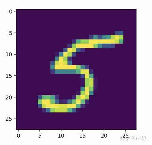
torch.Size([64]plt.imshow(images[0].numpy().squeeze())
让我们开始构建这个网络
inputs = images.view(images.shape[0],-1)
w1 = torch.randn(784, 256)
b1 = torch.randn(256)w2 = torch.randn(256, 10)
b2 = torch.randn(10)
h = activation(torch.mm(inputs, w1) + b1)
out = torch.mm(h, w2) + b2
torch.exp(x),dim=1参数说明了对于哪个维度去进行求和计算,由于我们的softmax是针对每一行的概率值求和,所以需要取第一个,view(-1,1) 将结果从1行64列转为64列一行,方便对没行进行softmax概率计算建议需要脑补两个向量互相作用,比较好理解
def softmax(x):return torch.exp(x) / torch.sum(torch.exp(x), dim=1).view(-1,1)
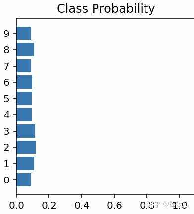
probabilities = softmax(out)# Does it have the right shape? Should be (64, 10)
print(probabilities.shape)
# Does it sum to 1?
print(probabilities.sum(dim=1))torch.Size([64, 10])
tensor([1.0000, 1.0000, 1.0000, 1.0000, 1.0000, 1.0000, 1.0000, 1.0000, 1.0000,1.0000, 1.0000, 1.0000, 1.0000, 1.0000, 1.0000, 1.0000, 1.0000, 1.0000,1.0000, 1.0000, 1.0000, 1.0000, 1.0000, 1.0000, 1.0000, 1.0000, 1.0000,1.0000, 1.0000, 1.0000, 1.0000, 1.0000, 1.0000, 1.0000, 1.0000, 1.0000,1.0000, 1.0000, 1.0000, 1.0000, 1.0000, 1.0000, 1.0000, 1.0000, 1.0000,1.0000, 1.0000, 1.0000, 1.0000, 1.0000, 1.0000, 1.0000, 1.0000, 1.0000,1.0000, 1.0000, 1.0000, 1.0000, 1.0000, 1.0000, 1.0000, 1.0000, 1.0000,1.0000])
nn模块进行网络构建。我们将构建一个输入784维,隐含层256维,10维度输出层的网络,并且结合softmax输出3.from torch import nn
class NetWork(nn.Module):def __init__(self):# 当需要继承父类构造函数中的内容# 且子类需要在父类的基础上补充时,使用super().__init__()super().__init__() # 定义隐层(输入维度,输出维度)self.hidden = nn.Linear(784,256)self.output = nn.Linear(256,10)# 定义激活函数self.sigmoid = nn.Sigmoid()self.softmax = nn.Softmax(1)def forward(self,x):# 定义前向反馈传播路径,x是输入向量,一层层的经过网络的洗礼x = self.hidden(x)x = self.sigmoid(x)x = self.output(x)x = self.softmax(x)return xmodel = NetWork()
modelNetWork((hidden): Linear(in_features=784, out_features=256, bias=True)(output): Linear(in_features=256, out_features=10, bias=True)(sigmoid): Sigmoid()(softmax): Softmax(dim=1)
)
我们也可以使用torch.nn.functional更简洁明了的定义网络。一般这种方式会比较常用
import torch.nn.functional as Fclass Network(nn.Module):def __init__(self):super().__init()self.hidden = nn.Linear(784,256)self.output = nn.Linear(256,10)def forward(self,x):x = F.sigmoid(self.hidden(x))x = F.softmax(self.output(x),dim=1)return x
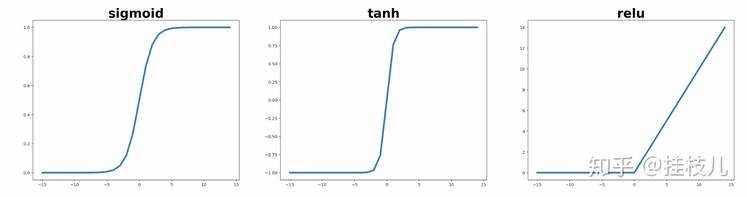
除了Softmax作为激活函数外,还有非常熟悉的Sigmoid函数,Tanh,和Relu都可以作为激活函数.(不过Relu赛高,因为Sigmoid的梯度在预测值较大,导致非常接近两端的时候,梯度很小,模型学习能力会受到很大的限制) 我们可以分别给激活函数画个图
x = np.arange(-15,15)
sigmoid = 1/(1+np.exp(-x))
tanh = 2/(1+np.exp(-2*x)) -1
relu = [i if i >=0 else 0 for i in x]fig,axes = plt.subplots(1,3,figsize=(30,7))
for ax,line,name in zip(axes,[sigmoid,tanh,relu],['sigmoid','tanh','relu']):ax.plot(x,line,lw=4)ax.set_title(name,fontsize=30,weight='bold')
根据晚上的教程,我们将构造一个784-128-64-10的神经网络,这一次我们加入激活函数
## Solutionclass Network(nn.Module):def __init__(self):super().__init__()# Defining the layers, 128, 64, 10 units eachself.fc1 = nn.Linear(784, 128)self.fc2 = nn.Linear(128, 64)# Output layer, 10 units - one for each digitself.fc3 = nn.Linear(64, 10)def forward(self, x):''' Forward pass through the network, returns the output logits '''x = self.fc1(x)x = F.relu(x)x = self.fc2(x)x = F.relu(x)x = self.fc3(x)x = F.softmax(x, dim=1)return xmodel = Network()
model
Network((fc1): Linear(in_features=784, out_features=128, bias=True)(fc2): Linear(in_features=128, out_features=64, bias=True)(fc3): Linear(in_features=64, out_features=10, bias=True)
)
model.fcx.weight来访问网络的这些属性.model.fc1.weight.shape
torch.Size([128, 784])model.fc1.bias.shape
torch.Size([128])model.fc1.bias.data.fill_(0)
tensor([0., 0., 0., 0., 0., 0., 0., 0., 0., 0., 0., 0., 0., 0., 0., 0., 0., 0., 0., 0., 0., 0., 0., 0.,0., 0., 0., 0., 0., 0., 0., 0., 0., 0., 0., 0., 0., 0., 0., 0., 0., 0., 0., 0., 0., 0., 0., 0.,0., 0., 0., 0., 0., 0., 0., 0., 0., 0., 0., 0., 0., 0., 0., 0., 0., 0., 0., 0., 0., 0., 0., 0.,0., 0., 0., 0., 0., 0., 0., 0., 0., 0., 0., 0., 0., 0., 0., 0., 0., 0., 0., 0., 0., 0., 0., 0.,0., 0., 0., 0., 0., 0., 0., 0., 0., 0., 0., 0., 0., 0., 0., 0., 0., 0., 0., 0., 0., 0., 0., 0.,0., 0., 0., 0., 0., 0., 0., 0.])model.fc1.weight.data.normal_(std=0.01)
tensor([[-0.0003, 0.0107, -0.0265, ..., -0.0097, 0.0048, -0.0024],[-0.0157, 0.0112, 0.0066, ..., -0.0172, -0.0062, 0.0107],[ 0.0022, 0.0017, -0.0013, ..., 0.0011, 0.0143, -0.0131],...,[ 0.0018, -0.0082, -0.0011, ..., -0.0071, -0.0085, 0.0081],[-0.0009, -0.0019, 0.0004, ..., -0.0051, 0.0110, 0.0013],[-0.0075, -0.0198, 0.0041, ..., -0.0231, -0.0113, 0.0050]])
构建完了网络,接下来我们让他往前跑起来!
dataiter = iter(trainloader)
images, labels = dataiter.next()# Resize images into a 1D vector, new shape is (batch size, color channels, image pixels)
images.resize_(64, 1, 784)s
img_idx = 0
ps = model.forward(images[img_idx,:])
nn.Sequential 构建模型 我真的不懂为啥要有那么多方式构建模型.....
input_size = 784
hidden_sizes = [128, 64]
output_size = 10model = nn.Sequential(nn.Linear(input_size, hidden_sizes[0]),nn.ReLU(),nn.Linear(hidden_sizes[0], hidden_sizes[1]),nn.ReLU(),nn.Linear(hidden_sizes[1], output_size),nn.Softmax(dim=1))
print(model)
Sequential((0): Linear(in_features=784, out_features=128, bias=True)(1): ReLU()(2): Linear(in_features=128, out_features=64, bias=True)(3): ReLU()(4): Linear(in_features=64, out_features=10, bias=True)(5): Softmax()
)images, labels = next(iter(trainloader))
images.resize_(images.shape[0], 1, 784)
ps = model.forward(images[0,:])
from collections import OrderedDictmodel = nn.Sequential(OrderedDict([('fc1', nn.Linear(input_size, hidden_sizes[0])),('relu1', nn.ReLU()),('fc2', nn.Linear(hidden_sizes[0], hidden_sizes[1])),('relu2', nn.ReLU()),('output', nn.Linear(hidden_sizes[1], output_size)),('softmax', nn.Softmax(dim=1))]))
modelSequential((fc1): Linear(in_features=784, out_features=128, bias=True)(relu1): ReLU()(fc2): Linear(in_features=128, out_features=64, bias=True)(relu2): ReLU()(output): Linear(in_features=64, out_features=10, bias=True)(softmax): Softmax()
)
print(model[0])
print(model.fc1)Linear(in_features=784, out_features=128, bias=True)
Linear(in_features=784, out_features=128, bias=True)


 京公网安备 11010802041100号 | 京ICP备19059560号-4 | PHP1.CN 第一PHP社区 版权所有