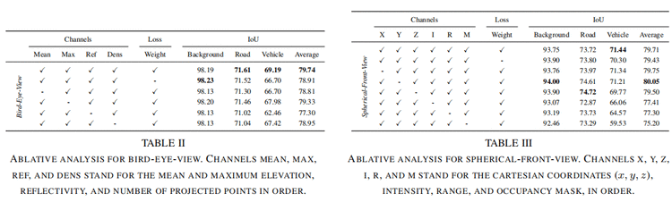
每个cell的编码:Similar to the work in 论文[4], in each grid cell, we compute the mean and maximum elevation, average reflectivity (i.e. intensity) value, and number of projected points.
Compared to 论文[4], we avoid using the minimum and standard deviation values of the height as additional features since our experiments showed that there is no significant contribution coming from those channels.
前视图
1)和SqueezeSeg一样的投射方式
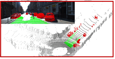
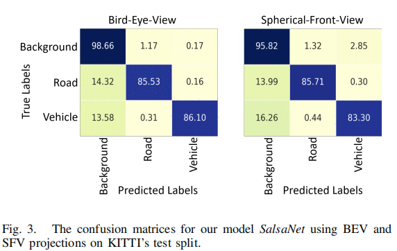
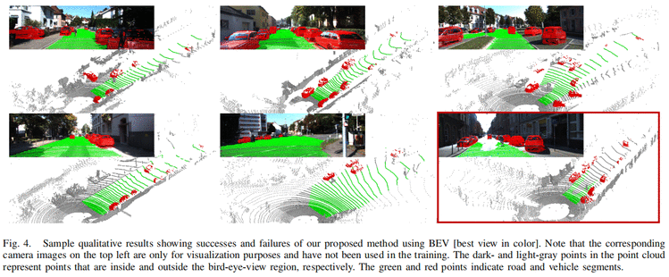
2)前视图一个不好的特性:遮挡,弯曲和变形:Although SFV returns more dense representation compared to BEV, SFV has certain distortion and deformation effects on small objects, e.g. vehicles. It is also more likely that objects in SFV tend to occlude each other. We, therefore, employ BEV representation as the main input to our network.
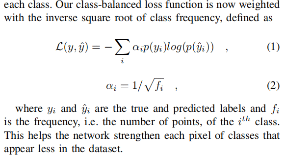
dropout放置的位置作者给出了说明,参考的是文献[26],We here emphasize that dropout needs to be placed right after batch normalization. As shown in [26], an early application of dropout can otherwise lead to a shift in the weight distribution and thus minimize the effect of batch normalization during training. 2.3 类别不平衡问题
用类别比例的开方作为loss weight的比例
2.4 训练超参数配置
数据增强的特殊方式: adding random pixel noise with probaility of 0.5, random rotation [-5,5]
3. 实验效果
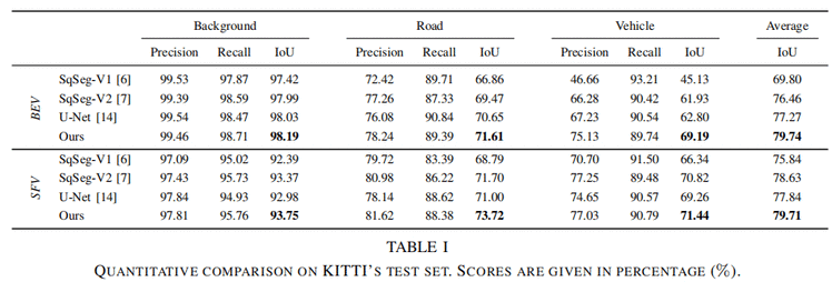
性能对比(外部)
俯视图和前视图的性能对比 (内部)
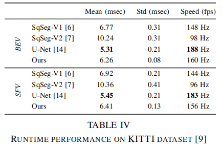
速度对比
4. 一些启示
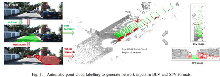
下面引用[11]需要学习一下, 如何半自动标注
这个论文的揭露了我们不一定把所有地面标出来,可以只标注freespace
这个论文loss weight的设计有一定参考价值
性能对比,不仅仅IOU, precision和recall的性能对比
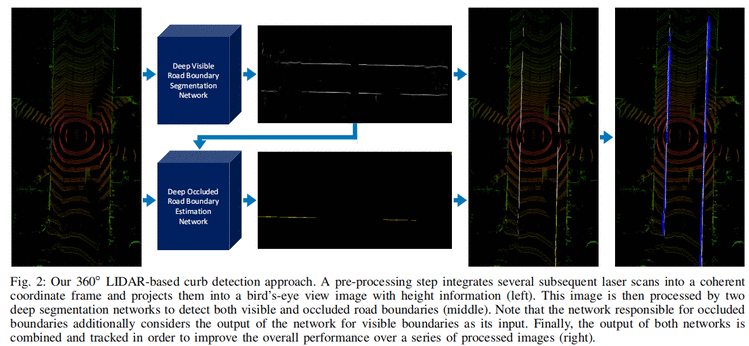
3. Online Inference and Detection of Curbs in Partially Occluded Scenes with Sparse LIDAR
[11] uses range and intensity information from 3D LIDAR to detect visible curbs on elevation data, which fails in the presence of occluding obstacles.
[12] presents a LIDAR-based method to detect visible curbs using sliding-beam segmentation followed by segment-specific curb detection, but fails to detect curbs behind obstacles.
如何生成路沿的曲线
In this work, we used images acquired by a Point Grey Bumblebee XB3 camera, mounted on the front of the platform facing towards the direction of motion. In particular, our implementation of VO uses FAST corners [16] combined with BRIEF descriptors [17], RANSAC [18] for outlier rejection, and nonlinear least-squares refinement.
将点的高度设置在3.55m内, 防止地上的水导致点云点特别低的情况。
将可视的线和遮挡的线进行分离
To determine which points are visible and which are occluded we use the hidden point removal operator as described in [20]. The operator determines all visible points in a pointcloud when observed from a given viewpoint. This is achieved by extracting all points residing on the convex hull of a transformed pointcloud. These points resemble the visible points, all other (labeled) points are considered as hidden (or occluded). We take the previously trimmed pointclouds and create binary bird’s-eye view images by taking the height of points from the ground into account. The points that are within a predefined height difference from the LIDAR roughly correspond to the points (obstacles) that are blocking the view. By putting together raw labels and binary masks of obstacles, obtained by running the hidden point removal algorithm, we obtain separate masks for visible and occluded road boundaries。(待了解)
网络结构
分析类Unet模型,不能很好检测处遮挡路沿的原因: first, the network’s limited receptive field, which is not big enough to capture context around large obstacles to estimate the position of curbs behind them, and second, the lack of structure (model-free) which prevents the network to infer very thin curves of occluded road boundaries within an image.
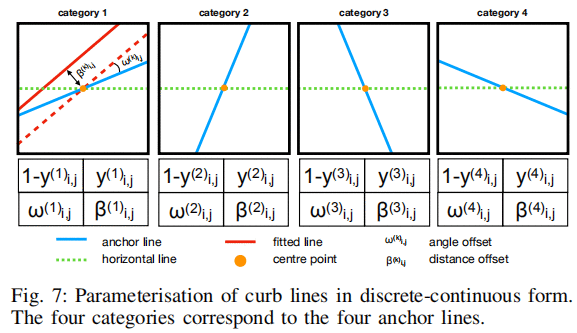
每个grid cell怎么预测这些线的?: Lines in each grid cell are parameterised in a discrete-continuous(离散且连续的线段) form: first, fitted lines are assigned to one of four types of anchor lines, and secondly, offsets between fitted and anchor lines are calculated. Anchor lines pass through the centre of a grid cell at different angles (22.5◦,67.5◦, 112.5◦and 157.5◦). During fitting, lines are assignedto the closest anchor line. Once a fitted line is discretised,two continuous parameters are calculated: (1) an angle offsetbetween a fitted and the respective anchor line ($w^k_{i,j,gy} ),and(2)adistancefromthecentreofthecelltothefittedline(), and (2) a distance from the centre of the cell to the fitted line (),and(2)adistancefromthecentreofthecelltothefittedline(β^k_{i, j,gt}$). As a result, we obtain 16 numbers for each grid cell, 4 numbers(w, β\betaβ, 类别-是否是线) for each line category.
To increase the receptive field of the model we added intra-layer convolutions [23] before the multi-scale parameter estimation layers. Traditional layer-by-layer convolutions are applied between feature maps, but intra-layer convolutions are slice-by-slice convolutions within feature maps. Hence, intra-layer convolutions capture aspects across the whole image and can thereby capture spatial relationships over longer distances. For example, there is a strong correlation between the length of the occluded curbs and the size of objects which are obstructing the view (ranging from 10-15 pixels through occlusions by traffic cones to 200-300 pixels through occlusions by several parked cars).
用交叉熵损失预测是否为路沿, 用smoothL1预测w,β\betaβ;
后处理
采用时间信息,也就是前后帧进行跟踪识别, 这样做有两个好处: filtering out false positives and tracking true positives.
filtering: we transform the last three output masks of detected road boundaries into a common reference attached to the current frame. Then we construct a histogram of output mask size (480x960) by counting the number of overlapping pixels with a value grater than threshold of 0.7 (which was determined experimentally). 可能如果这三帧的在同一个位置都有值的话,histogram会高,则保留; 否则则剔除该点。
Tracking. In the second step, we perform a similar procedure as outlined above. However, this time we consider road boundary masks from the last three frames that were generated by the first step (as shown in Figure 9). By taking the union of these masks we track the detected road boundaries over the time. Integrating temporal information helps to close gaps between boundary segments
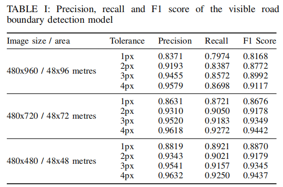
3. 实验效果
总结性能图
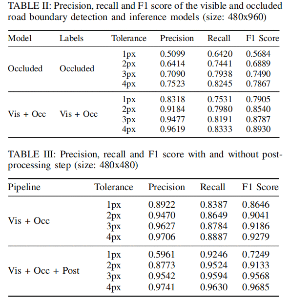
可见路沿和遮挡路沿的对比
添加后处理后的效果
4. 一些启示
直接预测路沿线的方法
用anchor line对遮挡的线进行预测
线的拟合思路: Fast corner【16】–> Brief descriptor[17]–>Ransac[18] for outlier rejection and nonlinear least-squares refinement.
官方提供了pts,intensity,category三类点云数据,我们这里参考了Complex-YOLO: Real-time 3D Object Detection on Point Clouds的思路将pts,intensity点云数据处理为最大反射强度,最大高度,归一化密度后再分别归一化到0~1的范围后重组为三通道图片数组,作为我们的训练图像。


 京公网安备 11010802041100号 | 京ICP备19059560号-4 | PHP1.CN 第一PHP社区 版权所有