火力发电就是燃料燃烧加热水生成蒸汽,蒸汽产生的压力推动汽轮机旋转,进而带动电机旋转,产生电能。其中一系列的能量转化中,影响发电效率的核心是锅炉的燃烧效率,即加热水产生的蒸汽量。而影响锅炉燃烧效率的因素很多,包括锅炉床温、床压、炉膛温度、压力等等。
这个赛题的目标就是给一堆锅炉传感器采集的数据(38个特征变量),然后用训练好的模型预测出蒸汽量。因为预测值为连续型数值变量,且给定的数据都带有标签,故此问题是典型的回归预测问题。
典型的回归预测模型使用的算法包括:线性回归,岭回归,LASSO回归,决策树回归,梯度提升树回归。
一个典型的机器学习实战算法基本包括 1) 数据处理,2) 特征选取、优化,和 3) 模型选取、验证、优化。 因为 “数据和特征决定了机器学习的上限,而模型和算法知识逼近这个上限而已。” 所以在解决一个机器学习问题时大部分时间都会花在数据处理和特征优化上。
大家最好在jupyter notebook上一段一段地跑下面的代码,加深理解。
机器学习的基本知识可以康康我的其他文章哦 好康的。
import warnings
warnings.filterwarnings("ignore")
import matplotlib.pyplot as plt
plt.rcParams.update({'figure.max_open_warning': 0})
import seaborn as sns
# modelling
import pandas as pd
import numpy as np
from scipy import stats
from sklearn.model_selection import train_test_split
from sklearn.model_selection import GridSearchCV, RepeatedKFold, cross_val_score,cross_val_predict,KFold
from sklearn.metrics import make_scorer,mean_squared_error
from sklearn.linear_model import LinearRegression, Lasso, Ridge, ElasticNet
from sklearn.svm import LinearSVR, SVR
from sklearn.neighbors import KNeighborsRegressor
from sklearn.ensemble import RandomForestRegressor, GradientBoostingRegressor,AdaBoostRegressor
from xgboost import XGBRegressor
from sklearn.preprocessing import PolynomialFeatures,MinMaxScaler,StandardScaler
#load_dataset
with open("./zhengqi_train.txt")  as fr:
    data_train=pd.read_table(fr,sep="\t")
with open("./zhengqi_test.txt") as fr_test:
    data_test=pd.read_table(fr_test,sep="\t")
#merge train_set and test_set
data_train["oringin"]="train"
data_test["oringin"]="test"
data_all=pd.concat([data_train,data_test],axis=0,ignore_index=True)
data_all.drop(["V5","V9","V11","V17","V22","V28"],axis=1,inplace=True)
# normalise numeric columns
cols_numeric=list(data_all.columns)
cols_numeric.remove("oringin")
def scale_minmax(col):
    return (col-col.min())/(col.max()-col.min())
scale_cols = [col for col in cols_numeric if col!='target']
data_all[scale_cols] = data_all[scale_cols].apply(scale_minmax,axis=0)
#Check effect of Box-Cox transforms on distributions of continuous variables
fcols = 6
frows = len(cols_numeric)-1
plt.figure(figsize=(4*fcols,4*frows))
i=0
for var in cols_numeric:
    if var!='target':
        dat = data_all[[var, 'target']].dropna()

        i+=1
        plt.subplot(frows,fcols,i)
        sns.distplot(dat[var] , fit=stats.norm);
        plt.title(var+' Original')
        plt.xlabel('')

        i+=1
        plt.subplot(frows,fcols,i)
        _=stats.probplot(dat[var], plot=plt)
        plt.title('skew='+'{:.4f}'.format(stats.skew(dat[var])))
        plt.xlabel('')
        plt.ylabel('')

        i+=1
        plt.subplot(frows,fcols,i)
        plt.plot(dat[var], dat['target'],'.',alpha=0.5)
        plt.title('corr='+'{:.2f}'.format(np.corrcoef(dat[var], dat['target'])[0][1]))

        i+=1
        plt.subplot(frows,fcols,i)
        trans_var, lambda_var = stats.boxcox(dat[var].dropna()+1)
        trans_var = scale_minmax(trans_var)
        sns.distplot(trans_var , fit=stats.norm);
        plt.title(var+' Tramsformed')
        plt.xlabel('')

        i+=1
        plt.subplot(frows,fcols,i)
        _=stats.probplot(trans_var, plot=plt)
        plt.title('skew='+'{:.4f}'.format(stats.skew(trans_var)))
        plt.xlabel('')
        plt.ylabel('')

        i+=1
        plt.subplot(frows,fcols,i)
        plt.plot(trans_var, dat['target'],'.',alpha=0.5)
        plt.title('corr='+'{:.2f}'.format(np.corrcoef(trans_var,dat['target'])[0][1]))
Box-Cox变换是Box和Cox在1964年提出的一种广义幂变换方法,是统计建模中常用的一种数据变换,用于连续的响应变量不满足正态分布的情况。Box-Cox变换之后,可以一定程度上减小不可观测的误差和预测变量的相关性。Box-Cox变换的主要特点是引入一个参数,通过数据本身估计该参数进而确定应采取的数据变换形式,Box-Cox变换可以明显地改善数据的正态性、对称性和方差相等性,对许多实际数据都是行之有效的。
cols_transform=data_all.columns[0:-2]
for col in cols_transform:
    # transform column
    data_all.loc[:,col], _ = stats.boxcox(data_all.loc[:,col]+1)
print(data_all.target.describe())
plt.figure(figsize=(12,4))
plt.subplot(1,2,1)
sns.distplot(data_all.target.dropna() , fit=stats.norm);
plt.subplot(1,2,2)
_=stats.probplot(data_all.target.dropna(), plot=plt)
#Log Transform SalePrice to improve normality
sp = data_train.target
data_train.target1 =np.power(1.5,sp)
print(data_train.target1.describe())
plt.figure(figsize=(12,4))
plt.subplot(1,2,1)
sns.distplot(data_train.target1.dropna(),fit=stats.norm);
plt.subplot(1,2,2)
_=stats.probplot(data_train.target1.dropna(), plot=plt)
# function to get training samples
def get_training_data():
    # extract training samples
    from sklearn.model_selection import train_test_split
    df_train = data_all[data_all["oringin"]=="train"]
    df_train["label"]=data_train.target1
    # split SalePrice and features
    y = df_train.target
    X = df_train.drop(["oringin","target","label"],axis=1)
    X_train,X_valid,y_train,y_valid=train_test_split(X,y,test_size=0.3,random_state=100)
    return X_train,X_valid,y_train,y_valid
# extract test data (without SalePrice)
def get_test_data():
    df_test = data_all[data_all["oringin"]=="test"].reset_index(drop=True)
    return df_test.drop(["oringin","target"],axis=1)
from sklearn.metrics import make_scorer
# metric for evaluation
def rmse(y_true, y_pred):
    diff = y_pred - y_true
    sum_sq = sum(diff**2)
    n = len(y_pred)

    return np.sqrt(sum_sq/n)
def mse(y_ture,y_pred):
    return mean_squared_error(y_ture,y_pred)
# scorer to be used in sklearn model fitting
rmse_scorer = make_scorer(rmse, greater_is_better=False)
mse_scorer = make_scorer(mse, greater_is_better=False)
# function to detect outliers based on the predictions of a model
def find_outliers(model, X, y, sigma=3):
    # predict y values using model
    try:
        y_pred = pd.Series(model.predict(X), index=y.index)
    # if predicting fails, try fitting the model first
    except:
        model.fit(X,y)
        y_pred = pd.Series(model.predict(X), index=y.index)

    # calculate residuals between the model prediction and true y values
    resid = y - y_pred
    mean_resid = resid.mean()
    std_resid = resid.std()
    # calculate z statistic, define outliers to be where |z|>sigma
    z = (resid - mean_resid)/std_resid
    outliers = z[abs(z)>sigma].index

    # print and plot the results
    print('R2=',model.score(X,y))
    print('rmse=',rmse(y, y_pred))
    print("mse=",mean_squared_error(y,y_pred))
    print('---------------------------------------')
    print('mean of residuals:',mean_resid)
    print('std of residuals:',std_resid)
    print('---------------------------------------')
    print(len(outliers),'outliers:')
    print(outliers.tolist())
    plt.figure(figsize=(15,5))
    ax_131 = plt.subplot(1,3,1)
    plt.plot(y,y_pred,'.')
    plt.plot(y.loc[outliers],y_pred.loc[outliers],'ro')
    plt.legend(['Accepted','Outlier'])
    plt.xlabel('y')
    plt.ylabel('y_pred');
    ax_132=plt.subplot(1,3,2)
    plt.plot(y,y-y_pred,'.')
    plt.plot(y.loc[outliers],y.loc[outliers]-y_pred.loc[outliers],'ro')
    plt.legend(['Accepted','Outlier'])
    plt.xlabel('y')
    plt.ylabel('y - y_pred');
    ax_133=plt.subplot(1,3,3)
    z.plot.hist(bins=50,ax=ax_133)
    z.loc[outliers].plot.hist(color='r',bins=50,ax=ax_133)
    plt.legend(['Accepted','Outlier'])
    plt.xlabel('z')

    plt.savefig('outliers.png')

    return outliers
# get training data
from sklearn.linear_model import Ridge
X_train, X_valid,y_train,y_valid = get_training_data()
test=get_test_data()
# find and remove outliers using a Ridge model
outliers = find_outliers(Ridge(), X_train, y_train)
# permanently remove these outliers from the data
#df_train = data_all[data_all["oringin"]=="train"]
#df_train["label"]=data_train.target1
#df_train=df_train.drop(outliers)
X_outliers=X_train.loc[outliers]
y_outliers=y_train.loc[outliers]
X_t=X_train.drop(outliers)
y_t=y_train.drop(outliers)

def get_trainning_data_omitoutliers():
    y1=y_t.copy()
    X1=X_t.copy()
    return X1,y1
from sklearn.preprocessing import StandardScaler
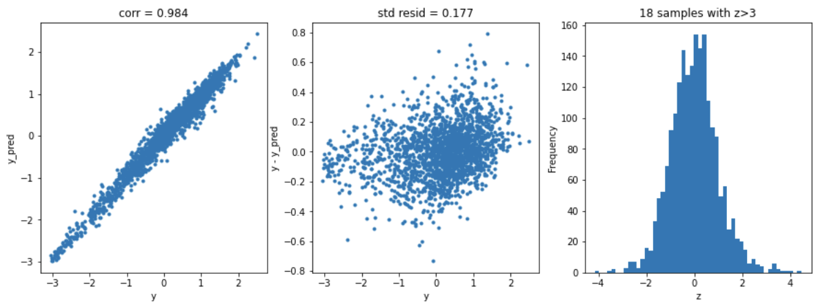
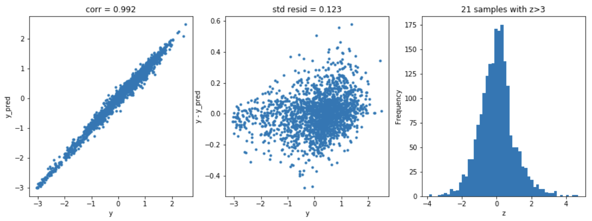
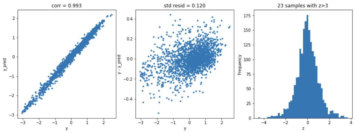
def train_model(model, param_grid=[], X=[], y=[],
splits=5, repeats=5):
# get unmodified training data, unless data to use already specified
if len(y)==0:
X,y = get_trainning_data_omitoutliers()
#poly_trans=PolynomialFeatures(degree=2)
#X=poly_trans.fit_transform(X)
#X=MinMaxScaler().fit_transform(X)
# create cross-validation method
rkfold = RepeatedKFold(n_splits=splits, n_repeats=repeats)
# perform a grid search if param_grid given
if len(param_grid)>0:
# setup grid search parameters
gsearch = GridSearchCV(model, param_grid, cv=rkfold,
scoring="neg_mean_squared_error",
verbose=1, return_train_score=True)
# search the grid
gsearch.fit(X,y)
# extract best model from the grid
model = gsearch.best_estimator_
best_idx = gsearch.best_index_
# get cv-scores for best model
grid_results = pd.DataFrame(gsearch.cv_results_)
cv_mean = abs(grid_results.loc[best_idx,'mean_test_score'])
cv_std = grid_results.loc[best_idx,'std_test_score']
# no grid search, just cross-val score for given model
else:
grid_results = []
cv_results = cross_val_score(model, X, y, scoring="neg_mean_squared_error", cv=rkfold)
cv_mean = abs(np.mean(cv_results))
cv_std = np.std(cv_results)
# combine mean and std cv-score in to a pandas series
cv_score = pd.Series({'mean':cv_mean,'std':cv_std})
# predict y using the fitted model
y_pred = model.predict(X)
# print stats on model performance
print('----------------------')
print(model)
print('----------------------')
print('score=',model.score(X,y))
print('rmse=',rmse(y, y_pred))
print('mse=',mse(y, y_pred))
print('cross_val: mean=',cv_mean,', std=',cv_std)
# residual plots
y_pred = pd.Series(y_pred,index=y.index)
resid = y - y_pred
mean_resid = resid.mean()
std_resid = resid.std()
z = (resid - mean_resid)/std_resid
n_outliers = sum(abs(z)>3)
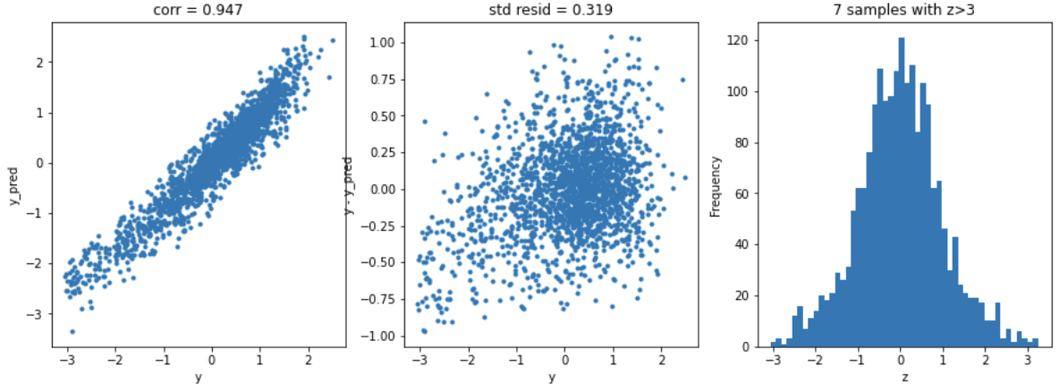
plt.figure(figsize=(15,5))
ax_131 = plt.subplot(1,3,1)
plt.plot(y,y_pred,'.')
plt.xlabel('y')
plt.ylabel('y_pred');
plt.title('corr = {:.3f}'.format(np.corrcoef(y,y_pred)[0][1]))
ax_132=plt.subplot(1,3,2)
plt.plot(y,y-y_pred,'.')
plt.xlabel('y')
plt.ylabel('y - y_pred');
plt.title('std resid = {:.3f}'.format(std_resid))
ax_133=plt.subplot(1,3,3)
z.plot.hist(bins=50,ax=ax_133)
plt.xlabel('z')
plt.title('{:.0f} samples with z>3'.format(n_outliers))
return model, cv_score, grid_results
# places to store optimal models and scores
opt_models = dict()
score_models = pd.DataFrame(columns=['mean','std'])
# no. k-fold splits
splits=5
# no. k-fold iterations
repeats=5
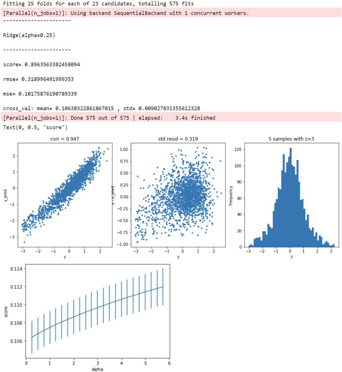
model = 'Ridge'
opt_models[model] = Ridge()
alph_range = np.arange(0.25,6,0.25)
param_grid = {'alpha': alph_range}
opt_models[model],cv_score,grid_results = train_model(opt_models[model], param_grid=param_grid,
                                              splits=splits, repeats=repeats)
cv_score.name = model
score_models = score_models.append(cv_score)
plt.figure()
plt.errorbar(alph_range, abs(grid_results['mean_test_score']),
             abs(grid_results['std_test_score'])/np.sqrt(splits*repeats))
plt.xlabel('alpha')
plt.ylabel('score')
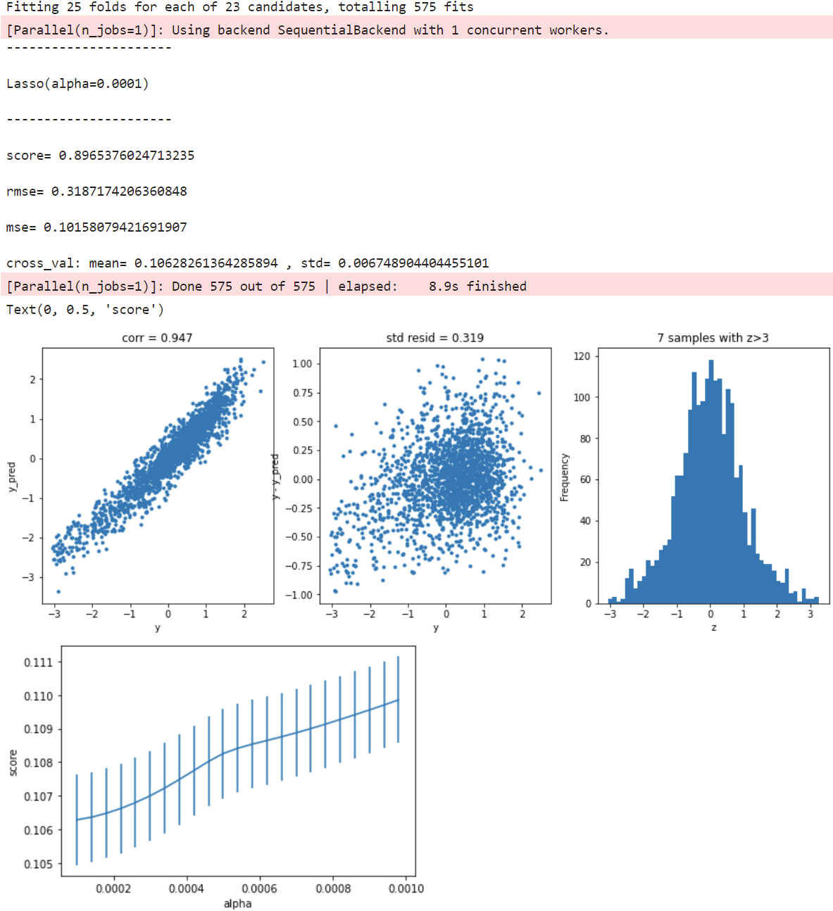
model = 'Lasso'
opt_models[model] = Lasso()
alph_range = np.arange(1e-4,1e-3,4e-5)
param_grid = {'alpha': alph_range}
opt_models[model], cv_score, grid_results = train_model(opt_models[model], param_grid=param_grid,
                                              splits=splits, repeats=repeats)
cv_score.name = model
score_models = score_models.append(cv_score)
plt.figure()
plt.errorbar(alph_range, abs(grid_results['mean_test_score']),abs(grid_results['std_test_score'])/np.sqrt(splits*repeats))
plt.xlabel('alpha')
plt.ylabel('score')
model ='ElasticNet'
opt_models[model] = ElasticNet()
param_grid = {'alpha': np.arange(1e-4,1e-3,1e-4),
              'l1_ratio': np.arange(0.1,1.0,0.1),
              'max_iter':[100000]}
opt_models[model], cv_score, grid_results = train_model(opt_models[model], param_grid=param_grid,
                                              splits=splits, repeats=1)
cv_score.name = model
score_models = score_models.append(cv_score)
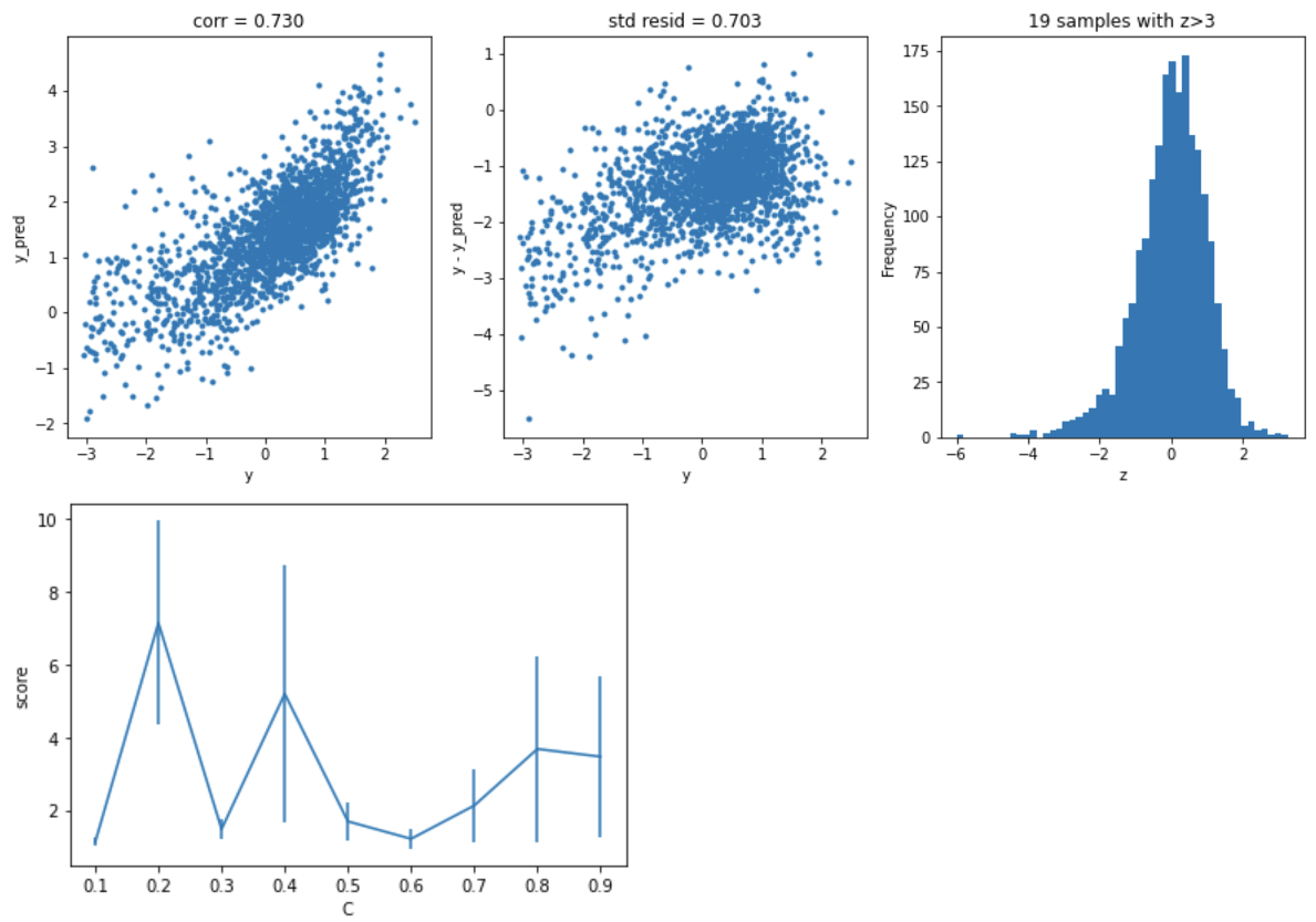
model='LinearSVR'
opt_models[model] = LinearSVR()
crange = np.arange(0.1,1.0,0.1)
param_grid = {'C':crange,
             'max_iter':[1000]}
opt_models[model], cv_score, grid_results = train_model(opt_models[model], param_grid=param_grid,
                                              splits=splits, repeats=repeats)
cv_score.name = model
score_models = score_models.append(cv_score)
plt.figure()
plt.errorbar(crange, abs(grid_results['mean_test_score']),abs(grid_results['std_test_score'])/np.sqrt(splits*repeats))
plt.xlabel('C')
plt.ylabel('score')
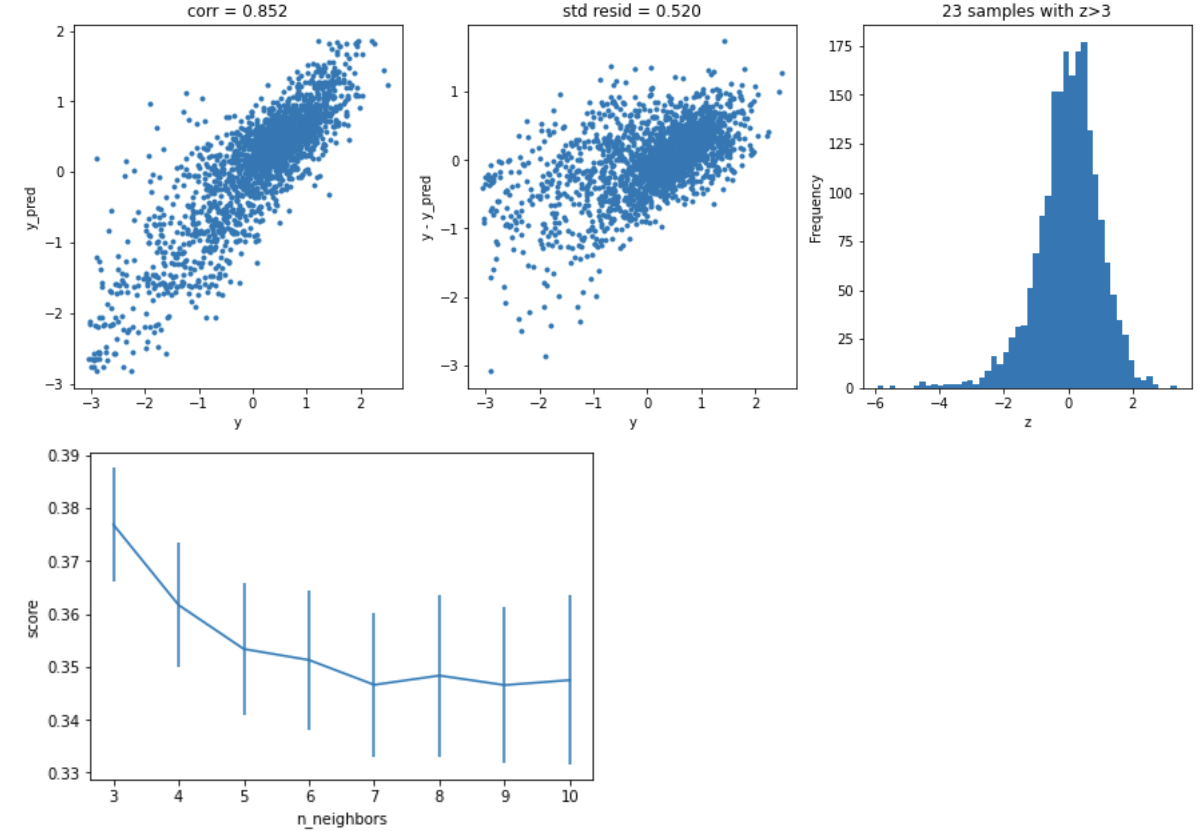
model = 'KNeighbors'
opt_models[model] = KNeighborsRegressor()
param_grid = {'n_neighbors':np.arange(3,11,1)}
opt_models[model], cv_score, grid_results = train_model(opt_models[model], param_grid=param_grid,
                                              splits=splits, repeats=1)
cv_score.name = model
score_models = score_models.append(cv_score)
plt.figure()
plt.errorbar(np.arange(3,11,1), abs(grid_results['mean_test_score']),abs(grid_results['std_test_score'])/np.sqrt(splits*1))
plt.xlabel('n_neighbors')
plt.ylabel('score')
model = 'GradientBoosting'
opt_models[model] = GradientBoostingRegressor()
param_grid = {'n_estimators':[150,250,350],
              'max_depth':[1,2,3],
              'min_samples_split':[5,6,7]}
opt_models[model], cv_score, grid_results = train_model(opt_models[model], param_grid=param_grid,
                                              splits=splits, repeats=1)
cv_score.name = model
score_models = score_models.append(cv_score)
model = 'XGB'
opt_models[model] = XGBRegressor()
param_grid = {'n_estimators':[100,200,300,400,500],
              'max_depth':[1,2,3],
             }
opt_models[model], cv_score,grid_results = train_model(opt_models[model], param_grid=param_grid,
                                              splits=splits, repeats=1)
cv_score.name = model
score_models = score_models.append(cv_score)
model = 'RandomForest'
opt_models[model] = RandomForestRegressor()
param_grid = {'n_estimators':[100,150,200],
              'max_features':[8,12,16,20,24],
              'min_samples_split':[2,4,6]}
opt_models[model], cv_score, grid_results = train_model(opt_models[model], param_grid=param_grid,
                                              splits=5, repeats=1)
cv_score.name = model
score_models = score_models.append(cv_score)
def model_predict(test_data,test_y=[],stack=False):
    #poly_trans=PolynomialFeatures(degree=2)
    #test_data1=poly_trans.fit_transform(test_data)
    #test_data=MinMaxScaler().fit_transform(test_data)
    i=0
    y_predict_total=np.zeros((test_data.shape[0],))
    for model in opt_models.keys():
        if model!="LinearSVR" and model!="KNeighbors":
            y_predict=opt_models[model].predict(test_data)
            y_predict_total+=y_predict
            i+=1
        if len(test_y)>0:
            print("{}_mse:".format(model),mean_squared_error(y_predict,test_y))
    y_predict_mean=np.round(y_predict_total/i,3)
    if len(test_y)>0:
        print("mean_mse:",mean_squared_error(y_predict_mean,test_y))
    else:
        y_predict_mean=pd.Series(y_predict_mean)
        return y_predict_mean
model_predict(X_valid,y_valid)

模型融合,即先产生一组个体模型,再用某种策略将它们结合起来,以加强模型效果。
分析表明,随着集成中个体模型数量T增加,集成模型的错误率将呈指数级下降,最终趋于0。通过融合可以达到取长补短的效果,综合个体模型的优势能降低预测误差、优化整体模型的性能。而且个体模型的准确率越高,多样性越大,模型融合的提升效果就越好!
import numpy as np
import matplotlib.pyplot as plt
import matplotlib.gridspec as gridspec
import itertools
from sklearn.linear_model import LogisticRegression
from sklearn.svm import SVC
from sklearn.ensemble import RandomForestClassifier
##主要使用pip install mlxtend安装mlxtend
from mlxtend.classifier import EnsembleVoteClassifier
from mlxtend.data import iris_data
from mlxtend.plotting import plot_decision_regions
%matplotlib inline
# Initializing Classifiers
clf1 = LogisticRegression(random_state=0)
clf2 = RandomForestClassifier(random_state=0)
clf3 = SVC(random_state=0, probability=True)
eclf = EnsembleVoteClassifier(clfs=[clf1, clf2, clf3], weights=[2, 1, 1], voting='soft')
# Loading some example data
X, y = iris_data()
X = X[:,[0, 2]]
# Plotting Decision Regions
gs = gridspec.GridSpec(2, 2)
fig = plt.figure(figsize=(10, 8))
for clf, lab, grd in zip([clf1, clf2, clf3, eclf],
                         ['Logistic Regression', 'Random Forest', 'RBF kernel SVM', 'Ensemble'],
                         itertools.product([0, 1], repeat=2)):
    clf.fit(X, y)
    ax = plt.subplot(gs[grd[0], grd[1]])
    fig = plot_decision_regions(X=X, y=y, clf=clf, legend=2)
    plt.title(lab)
plt.show()

from sklearn.model_selection import train_test_split
import pandas as pd
import numpy as np
from scipy import sparse
import xgboost
import lightgbm
from sklearn.ensemble import RandomForestRegressor,AdaBoostRegressor,GradientBoostingRegressor,ExtraTreesRegressor
from sklearn.linear_model import LinearRegression
from sklearn.metrics import mean_squared_error
def stacking_reg(clf,train_x,train_y,test_x,clf_name,kf,label_split=None):
    train=np.zeros((train_x.shape[0],1))
    test=np.zeros((test_x.shape[0],1))
    test_pre=np.empty((folds,test_x.shape[0],1))
    cv_scores=[]
    for i,(train_index,test_index) in enumerate(kf.split(train_x,label_split)):
        tr_x=train_x[train_index]
        tr_y=train_y[train_index]
        te_x=train_x[test_index]
        te_y = train_y[test_index]
        if clf_name in ["rf","ada","gb","et","lr","lsvc","knn"]:
            clf.fit(tr_x,tr_y)
            pre=clf.predict(te_x).reshape(-1,1)
            train[test_index]=pre
            test_pre[i,:]=clf.predict(test_x).reshape(-1,1)
            cv_scores.append(mean_squared_error(te_y, pre))
        elif clf_name in ["xgb"]:
            train_matrix = clf.DMatrix(tr_x, label=tr_y, missing=-1)
            test_matrix = clf.DMatrix(te_x, label=te_y, missing=-1)
            z = clf.DMatrix(test_x, label=te_y, missing=-1)
            params = {'booster': 'gbtree',
                      'eval_metric': 'rmse',
                      'gamma': 1,
                      'min_child_weight': 1.5,
                      'max_depth': 5,
                      'lambda': 10,
                      'subsample': 0.7,
                      'colsample_bytree': 0.7,
                      'colsample_bylevel': 0.7,
                      'eta': 0.03,
                      'tree_method': 'exact',
                      'seed': 2017,
                      'nthread': 12
                      }
            num_round = 10000
            early_stopping_rounds = 100
            watchlist = [(train_matrix, 'train'),
                         (test_matrix, 'eval')
                         ]
            if test_matrix:
                model = clf.train(params, train_matrix, num_boost_round=num_round,evals=watchlist,
                                  early_stopping_rounds=early_stopping_rounds
                                  )
                pre= model.predict(test_matrix,ntree_limit=model.best_ntree_limit).reshape(-1,1)
                train[test_index]=pre
                test_pre[i, :]= model.predict(z, ntree_limit=model.best_ntree_limit).reshape(-1,1)
                cv_scores.append(mean_squared_error(te_y, pre))
        elif clf_name in ["lgb"]:
            train_matrix = clf.Dataset(tr_x, label=tr_y)
            test_matrix = clf.Dataset(te_x, label=te_y)
            #z = clf.Dataset(test_x, label=te_y)
            #z=test_x
            params = {
                      'boosting_type': 'gbdt',
                      'objective': 'regression_l2',
                      'metric': 'mse',
                      'min_child_weight': 1.5,
                      'num_leaves': 2**5,
                      'lambda_l2': 10,
                      'subsample': 0.7,
                      'colsample_bytree': 0.7,
                      'colsample_bylevel': 0.7,
                      'learning_rate': 0.03,
                      'tree_method': 'exact',
                      'seed': 2017,
                      'nthread': 12,
                      'silent': True,
                      }
            num_round = 10000
            early_stopping_rounds = 100
            if test_matrix:
                model = clf.train(params, train_matrix,num_round,valid_sets=test_matrix,
                                  early_stopping_rounds=early_stopping_rounds
                                  )
                pre= model.predict(te_x,num_iteration=model.best_iteration).reshape(-1,1)
                train[test_index]=pre
                test_pre[i, :]= model.predict(test_x, num_iteration=model.best_iteration).reshape(-1,1)
                cv_scores.append(mean_squared_error(te_y, pre))
        else:
            raise IOError("Please add new clf.")
        print("%s now score is:"%clf_name,cv_scores)
    test[:]=test_pre.mean(axis=0)
    print("%s_score_list:"%clf_name,cv_scores)
    print("%s_score_mean:"%clf_name,np.mean(cv_scores))
    return train.reshape(-1,1),test.reshape(-1,1)
def rf_reg(x_train, y_train, x_valid, kf, label_split=None):
    randomforest = RandomForestRegressor(n_estimators=600, max_depth=20, n_jobs=-1, random_state=2017, max_features="auto",verbose=1)
    rf_train, rf_test = stacking_reg(randomforest, x_train, y_train, x_valid, "rf", kf, label_split=label_split)
    return rf_train, rf_test,"rf_reg"
def ada_reg(x_train, y_train, x_valid, kf, label_split=None):
    adaboost = AdaBoostRegressor(n_estimators=30, random_state=2017, learning_rate=0.01)
    ada_train, ada_test = stacking_reg(adaboost, x_train, y_train, x_valid, "ada", kf, label_split=label_split)
    return ada_train, ada_test,"ada_reg"
def gb_reg(x_train, y_train, x_valid, kf, label_split=None):
    gbdt = GradientBoostingRegressor(learning_rate=0.04, n_estimators=100, subsample=0.8, random_state=2017,max_depth=5,verbose=1)
    gbdt_train, gbdt_test = stacking_reg(gbdt, x_train, y_train, x_valid, "gb", kf, label_split=label_split)
    return gbdt_train, gbdt_test,"gb_reg"
def et_reg(x_train, y_train, x_valid, kf, label_split=None):
    extratree = ExtraTreesRegressor(n_estimators=600, max_depth=35, max_features="auto", n_jobs=-1, random_state=2017,verbose=1)
    et_train, et_test = stacking_reg(extratree, x_train, y_train, x_valid, "et", kf, label_split=label_split)
    return et_train, et_test,"et_reg"
def lr_reg(x_train, y_train, x_valid, kf, label_split=None):
    lr_reg=LinearRegression(n_jobs=-1)
    lr_train, lr_test = stacking_reg(lr_reg, x_train, y_train, x_valid, "lr", kf, label_split=label_split)
    return lr_train, lr_test, "lr_reg"
def xgb_reg(x_train, y_train, x_valid, kf, label_split=None):
    xgb_train, xgb_test = stacking_reg(xgboost, x_train, y_train, x_valid, "xgb", kf, label_split=label_split)
    return xgb_train, xgb_test,"xgb_reg"
def lgb_reg(x_train, y_train, x_valid, kf, label_split=None):
    lgb_train, lgb_test = stacking_reg(lightgbm, x_train, y_train, x_valid, "lgb", kf, label_split=label_split)
    return lgb_train, lgb_test,"lgb_reg"
def stacking_pred(x_train, y_train, x_valid, kf, clf_list, label_split=None, clf_fin="lgb", if_concat_origin=True):
    for k, clf_list in enumerate(clf_list):
        clf_list = [clf_list]
        column_list = []
        train_data_list=[]
        test_data_list=[]
        for clf in clf_list:
            train_data,test_data,clf_name=clf(x_train, y_train, x_valid, kf, label_split=label_split)
            train_data_list.append(train_data)
            test_data_list.append(test_data)
            column_list.append("clf_%s" % (clf_name))
    train = np.concatenate(train_data_list, axis=1)
    test = np.concatenate(test_data_list, axis=1)

    if if_concat_origin:
        train = np.concatenate([x_train, train], axis=1)
        test = np.concatenate([x_valid, test], axis=1)
    print(x_train.shape)
    print(train.shape)
    print(clf_name)
    print(clf_name in ["lgb"])
    if clf_fin in ["rf","ada","gb","et","lr","lsvc","knn"]:
        if clf_fin in ["rf"]:
            clf = RandomForestRegressor(n_estimators=600, max_depth=20, n_jobs=-1, random_state=2017, max_features="auto",verbose=1)
        elif clf_fin in ["ada"]:
            clf = AdaBoostRegressor(n_estimators=30, random_state=2017, learning_rate=0.01)
        elif clf_fin in ["gb"]:
            clf = GradientBoostingRegressor(learning_rate=0.04, n_estimators=100, subsample=0.8, random_state=2017,max_depth=5,verbose=1)
        elif clf_fin in ["et"]:
            clf = ExtraTreesRegressor(n_estimators=600, max_depth=35, max_features="auto", n_jobs=-1, random_state=2017,verbose=1)
        elif clf_fin in ["lr"]:
            clf = LinearRegression(n_jobs=-1)
        clf.fit(train, y_train)
        pre = clf.predict(test).reshape(-1,1)
        return pred
    elif clf_fin in ["xgb"]:
        clf = xgboost
        train_matrix = clf.DMatrix(train, label=y_train, missing=-1)
        test_matrix = clf.DMatrix(train, label=y_train, missing=-1)
        params = {'booster': 'gbtree',
                  'eval_metric': 'rmse',
                  'gamma': 1,
                  'min_child_weight': 1.5,
                  'max_depth': 5,
                  'lambda': 10,
                  'subsample': 0.7,
                  'colsample_bytree': 0.7,
                  'colsample_bylevel': 0.7,
                  'eta': 0.03,
                  'tree_method': 'exact',
                  'seed': 2017,
                  'nthread': 12
                  }
        num_round = 10000
        early_stopping_rounds = 100
        watchlist = [(train_matrix, 'train'),
                     (test_matrix, 'eval')
                     ]
        model = clf.train(params, train_matrix, num_boost_round=num_round,evals=watchlist,
                          early_stopping_rounds=early_stopping_rounds
                          )
        pre = model.predict(test,ntree_limit=model.best_ntree_limit).reshape(-1,1)
        return pre
    elif clf_fin in ["lgb"]:
        print(clf_name)
        clf = lightgbm
        train_matrix = clf.Dataset(train, label=y_train)
        test_matrix = clf.Dataset(train, label=y_train)
        params = {
                  'boosting_type': 'gbdt',
                  'objective': 'regression_l2',
                  'metric': 'mse',
                  'min_child_weight': 1.5,
                  'num_leaves': 2**5,
                  'lambda_l2': 10,
                  'subsample': 0.7,
                  'colsample_bytree': 0.7,
                  'colsample_bylevel': 0.7,
                  'learning_rate': 0.03,
                  'tree_method': 'exact',
                  'seed': 2017,
                  'nthread': 12,
                  'silent': True,
                  }
        num_round = 10000
        early_stopping_rounds = 100
        model = clf.train(params, train_matrix,num_round,valid_sets=test_matrix,
                          early_stopping_rounds=early_stopping_rounds
                          )
        print('pred')
        pre = model.predict(test,num_iteration=model.best_iteration).reshape(-1,1)
        print(pre)
        return pre
# #load_dataset
with open("./zhengqi_train.txt")  as fr:
    data_train=pd.read_table(fr,sep="\t")
with open("./zhengqi_test.txt") as fr_test:
    data_test=pd.read_table(fr_test,sep="\t")
from sklearn.model_selection import StratifiedKFold, KFold
folds = 5
seed = 1
kf = KFold(n_splits=5, shuffle=True, random_state=0)
x_train = data_train[data_test.columns].values
x_valid = data_test[data_test.columns].values
y_train = data_train['target'].values
clf_list = [lr_reg, lgb_reg]
#clf_list = [lr_reg, rf_reg]
##很容易过拟合
pred = stacking_pred(x_train, y_train, x_valid, kf, clf_list, label_split=None, clf_fin="lgb", if_concat_origin=True)
以上内容和代码全部来自于《阿里云天池大赛赛题解析(机器学习篇)》这本好书,十分推荐大家去阅读原书!


 京公网安备 11010802041100号 | 京ICP备19059560号-4 | PHP1.CN 第一PHP社区 版权所有